9.7. 演習・Twitterのテキスト分類問題

実データを用いて機械学習を用いた分類問題を実践例として、Twitter投稿データの分類問題を考えます。

（ここでは、2020年に収集したデータを用います）

国内政治家アカウントのうち、データ収集時に最もフォロワー数がいる2人（橋下徹 @hashimoto_lo 安倍晋三 @AbeShinzo）のツイートをそれぞれどのユーザーの発信によるものか分類してみましょう。

import pandas as pd
import pickle
import numpy as np
from matplotlib import pyplot as plt
import japanize_matplotlib
%matplotlib inline
pd.set_option('display.max_columns', 100)

dfs = []
for user in ['hashimoto_lo','AbeShinzo']:
    with open('./data/tweets_{}.pkl'.format(user), 'rb') as f:
        tmp = pickle.load(f)
        dfs.append(tmp)

df = pd.concat(dfs)

df.info()

<class 'pandas.core.frame.DataFrame'>
Index: 5284 entries, 0 to 2067
Data columns (total 29 columns):
 #   Column                     Non-Null Count  Dtype  
---  ------                     --------------  -----  
 0   contributors               0 non-null      object 
 1   coordinates                0 non-null      object 
 2   created_at                 5284 non-null   object 
 3   entities                   5284 non-null   object 
 4   extended_entities          674 non-null    object 
 5   favorite_count             5284 non-null   int64  
 6   favorited                  5284 non-null   bool   
 7   geo                        0 non-null      object 
 8   id                         5284 non-null   int64  
 9   id_str                     5284 non-null   object 
 10  in_reply_to_screen_name    812 non-null    object 
 11  in_reply_to_status_id      810 non-null    float64
 12  in_reply_to_status_id_str  810 non-null    object 
 13  in_reply_to_user_id        812 non-null    float64
 14  in_reply_to_user_id_str    812 non-null    object 
 15  is_quote_status            5284 non-null   bool   
 16  lang                       5284 non-null   object 
 17  place                      1 non-null      object 
 18  possibly_sensitive         3521 non-null   object 
 19  quoted_status              782 non-null    object 
 20  quoted_status_id           1017 non-null   float64
 21  quoted_status_id_str       1017 non-null   object 
 22  retweet_count              5284 non-null   int64  
 23  retweeted                  5284 non-null   bool   
 24  retweeted_status           1040 non-null   object 
 25  source                     5284 non-null   object 
 26  text                       5284 non-null   object 
 27  truncated                  5284 non-null   bool   
 28  user                       5284 non-null   object 
dtypes: bool(4), float64(3), int64(3), object(19)
memory usage: 1.1+ MB

df.head(5)

	contributors	coordinates	created_at	entities	extended_entities	favorite_count	favorited	geo	id	id_str	in_reply_to_screen_name	in_reply_to_status_id	in_reply_to_status_id_str	in_reply_to_user_id	in_reply_to_user_id_str	is_quote_status	lang	place	possibly_sensitive	quoted_status	quoted_status_id	quoted_status_id_str	retweet_count	retweeted	retweeted_status	source	text	truncated	user
0	None	None	Sun Aug 02 22:39:43 +0000 2020	{'hashtags': [], 'symbols': [], 'user_mentions...	NaN	399	False	None	1290054702210531329	1290054702210531329	None	NaN	None	NaN	None	False	ja	None	False	NaN	NaN	NaN	44	False	NaN	<a href="http://twitter.com/download/android" ...	（スタッフよりお知らせ）本日13:55より生放送「情報ライブ　ミヤネ屋」（読売テレビ）に、橋...	False	{'id': 245677083, 'id_str': '245677083', 'name...
1	None	None	Sat Aug 01 15:49:14 +0000 2020	{'hashtags': [{'text': '日曜報道THEPRIME', 'indice...	NaN	0	False	None	1289589012785586176	1289589012785586176	None	NaN	None	NaN	None	False	ja	None	NaN	NaN	NaN	NaN	98	False	{'created_at': 'Sat Aug 01 15:14:22 +0000 2020...	<a href="http://twitter.com/download/iphone" r...	RT @THEPRIME_CX: 今日の #日曜報道THEPRIME は...【感染列島８月...	False	{'id': 245677083, 'id_str': '245677083', 'name...
2	None	None	Sat Aug 01 13:45:07 +0000 2020	{'hashtags': [], 'symbols': [], 'user_mentions...	NaN	1693	False	None	1289557775266136064	1289557775266136064	hashimoto_lo	1.289558e+18	1289557773630414850	245677083.0	245677083	False	ja	None	NaN	NaN	NaN	NaN	189	False	NaN	<a href="http://twitter.com/download/iphone" r...	評論家には政治はできません。ただうまくメッセージを出せない政治家も多いでしょう。政治に評論家...	False	{'id': 245677083, 'id_str': '245677083', 'name...
3	None	None	Sat Aug 01 13:45:06 +0000 2020	{'hashtags': [], 'symbols': [], 'user_mentions...	NaN	1341	False	None	1289557773630414850	1289557773630414850	None	NaN	None	NaN	None	True	ja	None	False	{'created_at': 'Sat Aug 01 07:14:22 +0000 2020...	1.289459e+18	1289459440555450369	131	False	NaN	<a href="http://twitter.com/download/iphone" r...	それは党内の政治事情ですね。このような場合、僕が代表だったときには、有権者には「本来この特措...	True	{'id': 245677083, 'id_str': '245677083', 'name...
4	None	None	Sat Aug 01 12:00:34 +0000 2020	{'hashtags': [], 'symbols': [], 'user_mentions...	NaN	749	False	None	1289531464892088320	1289531464892088320	None	NaN	None	NaN	None	False	ja	None	False	NaN	NaN	NaN	67	False	NaN	<a href="https://abema.tv" rel="nofollow">ABEM...	NewsBAR橋下、始まりました！（スタッフより） @ABEMA で視聴中 https://...	False	{'id': 245677083, 'id_str': '245677083', 'name...

df['user_name'] = df['user'].apply(lambda x: x['name'])

df = df.drop_duplicates(['id'])

df['user_screen_name'] = df['user'].apply(lambda x: x['screen_name'])

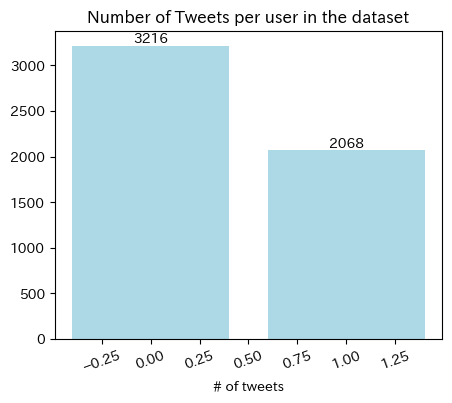
9.7.1. 全期間におけるユーザー別ツイート数

fig, ax = plt.subplots(1,1,figsize= (5,4))
N_tweets_users = df['user_screen_name'].value_counts().to_frame().reset_index().sort_values(by = 'user_screen_name', ascending=False)
bars = plt.bar(N_tweets_users.index, N_tweets_users['count'], color = 'lightblue')
ax.bar_label(bars)
plt.title('Number of Tweets per user in the dataset')
plt.xlabel('# of tweets')
plt.xticks(rotation=20)
plt.show()

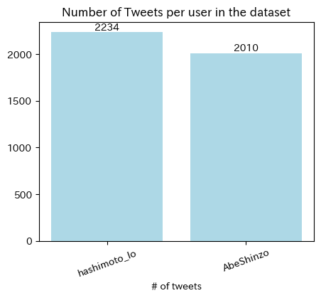
分析対象はRetweetでは無いオリジナルのTweetsのみとする

df = df[df['retweeted_status'].isnull()]

print(df.shape)

(4244, 31)

fig, ax = plt.subplots(1,1,figsize= (5,4))
N_tweets_users = df['user_screen_name'].value_counts().to_frame().sort_values(by = 'user_screen_name', ascending=False)
bars = plt.bar(N_tweets_users.index, N_tweets_users['count'], color = 'lightblue')
ax.bar_label(bars)
plt.title('Number of Tweets per user in the dataset')
plt.xlabel('# of tweets')
plt.xticks(rotation=20)
plt.show()

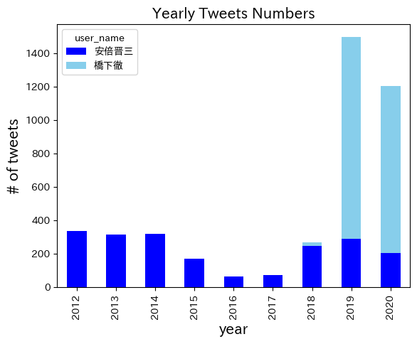
9.7.2. 年別のツイート数

df['created_at'] = pd.to_datetime(df['created_at'])
df['date'] = df['created_at'].dt.date
df['year'] = df['created_at'].dt.year
df['time'] = df['created_at'].dt.time

/var/folders/z5/0lnyp_m54dqc1xkz22ncbj2h0000gn/T/ipykernel_33116/1336334527.py:1: UserWarning: Could not infer format, so each element will be parsed individually, falling back to `dateutil`. To ensure parsing is consistent and as-expected, please specify a format.
  df['created_at'] = pd.to_datetime(df['created_at'])

df.head(1)

	contributors	coordinates	created_at	entities	extended_entities	favorite_count	favorited	geo	id	id_str	in_reply_to_screen_name	in_reply_to_status_id	in_reply_to_status_id_str	in_reply_to_user_id	in_reply_to_user_id_str	is_quote_status	lang	place	possibly_sensitive	quoted_status	quoted_status_id	quoted_status_id_str	retweet_count	retweeted	retweeted_status	source	text	truncated	user	user_name	user_screen_name	date	year	time
0	None	None	2020-08-02 22:39:43+00:00	{'hashtags': [], 'symbols': [], 'user_mentions...	NaN	399	False	None	1290054702210531329	1290054702210531329	None	NaN	None	NaN	None	False	ja	None	False	NaN	NaN	NaN	44	False	NaN	<a href="http://twitter.com/download/android" ...	（スタッフよりお知らせ）本日13:55より生放送「情報ライブ　ミヤネ屋」（読売テレビ）に、橋...	False	{'id': 245677083, 'id_str': '245677083', 'name...	橋下徹	hashimoto_lo	2020-08-02	2020	22:39:43

pd.crosstab(df['user_name'],df['year'])

year	2012	2013	2014	2015	2016	2017	2018	2019	2020
user_name
安倍晋三	336	315	318	168	62	73	247	288	203
橋下徹	0	0	0	0	0	0	21	1212	1001

pd.crosstab(df['user_name'],df['year']).T.plot.bar(stacked=True, color=['blue','skyblue'])
plt.title('Yearly Tweets Numbers', fontsize=15)
plt.xlabel('year', fontsize=15)
plt.ylabel('# of tweets', fontsize=15)
plt.show()

9.7.3. ユーザー別のLikesのヒストグラム

import matplotlib.pyplot as plt

fig, ax = plt.subplots(1,1, figsize=(5,3))

for i, arr in enumerate(df.groupby(['user_screen_name'])['favorite_count']):
    ax.hist(arr[1], bins = 100, 
            color=['blue','skyblue'][i], alpha = .7, label = arr[0])
plt.legend()
plt.title('Histgram of likes per user', fontsize=15)
plt.ylabel('Frequency', fontsize=13)
plt.xlabel('Number of Likes', fontsize=13)
plt.show()

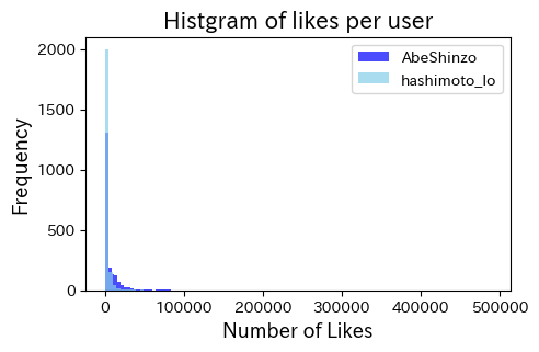
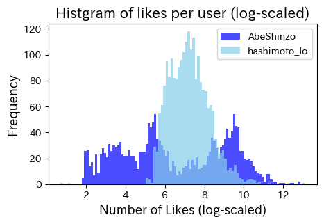
上の図では少しわかりにくいので、対数変換値をプロット

fig, ax = plt.subplots(1,1, figsize=(5,3))
for i, arr in enumerate(df.groupby(['user_screen_name'])['favorite_count']):
    ax.hist(arr[1].apply(lambda x: np.log(x)), bins = 100, 
            color=['blue','skyblue'][i], alpha = .7, label = arr[0])
plt.legend()
plt.title('Histgram of likes per user (log-scaled)', fontsize=15)
plt.ylabel('Frequency', fontsize=13)
plt.xlabel('Number of Likes (log-scaled)', fontsize=13)
plt.show()

9.7.4. ユーザー別のRetweetされた数のヒストグラム

fig, ax = plt.subplots(1,1, figsize=(5,3))

for i, arr in enumerate(df.groupby(['user_screen_name'])['retweet_count']):
    ax.hist(arr[1], bins = 100, 
            color=['blue','skyblue'][i], alpha = .7, label = arr[0])
plt.legend()
plt.title('Histgram of retweet per user', fontsize=15)
plt.ylabel('Frequency', fontsize=13)
plt.xlabel('Number of retweet', fontsize=13)
plt.show()

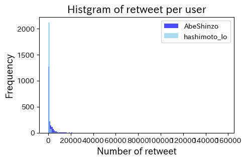
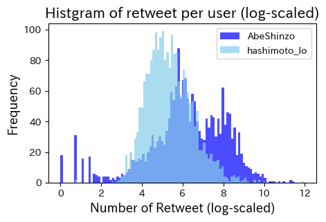
上の図では少しわかりにくいので、対数変換値をプロット

fig, ax = plt.subplots(1,1, figsize=(5,3))
for i, arr in enumerate(df.groupby(['user_screen_name'])['retweet_count']):
    ax.hist(arr[1].apply(lambda x: np.log(1+x)), bins = 100, 
            color=['blue','skyblue'][i], alpha = .7, label = arr[0])
plt.legend()
plt.title('Histgram of retweet per user (log-scaled)', fontsize=15)
plt.ylabel('Frequency', fontsize=13)
plt.xlabel('Number of Retweet (log-scaled)', fontsize=13)
plt.show()

9.7.5. 日本語の正規化（表記ゆれの是正）と形態素解析を行う

9.7.5.1. 正規化

1. 正規化を自動で実施してくれるパッケージをインストール。Terminal or Anaconda Prompt で　pip install neologdn

2. import nelogdn neologdn.normalize() で正規化

3. Regular ExpressionでテキストからURLを除外する

9.7.5.2. 形態素解析

1. pip install janome

from janome.tokenizer import Tokenizer
import neologdn
import re
from sklearn.feature_extraction.text import CountVectorizer
from sklearn.feature_extraction.text import TfidfVectorizer
from sklearn.model_selection import train_test_split
from sklearn.linear_model import LogisticRegression
from sklearn.metrics import classification_report
from sklearn import metrics
from sklearn.metrics import roc_auc_score
from sklearn.metrics import roc_curve
from sklearn.ensemble import RandomForestClassifier
from sklearn import svm
import sklearn as sk
from sklearn.neural_network import MLPClassifier
from sklearn.decomposition import PCA
from sklearn.cluster import MiniBatchKMeans
import itertools, random

正規化

df.loc[:,'standarized_text'] = df['text'].apply(lambda x: neologdn.normalize(x))

pat = re.compile(r'https?://\S+')
df.loc[:, 'standarized_text'] = df['standarized_text'].apply(lambda x: re.sub(pat, '', x))

# neologd_tagger = MeCab.Tagger('-Ochasen -d /opt/homebrew/lib/mecab/dic/mecab-ipadic-neologd')
t = Tokenizer()
for token in t.tokenize('庭には二羽鶏がいる'):
    print(token)

庭	名詞,一般,*,*,*,*,庭,ニワ,ニワ
に	助詞,格助詞,一般,*,*,*,に,ニ,ニ
は	助詞,係助詞,*,*,*,*,は,ハ,ワ
二	名詞,数,*,*,*,*,二,ニ,ニ
羽	名詞,接尾,助数詞,*,*,*,羽,ワ,ワ
鶏	名詞,一般,*,*,*,*,鶏,ニワトリ,ニワトリ
が	助詞,格助詞,一般,*,*,*,が,ガ,ガ
いる	動詞,自立,*,*,一段,基本形,いる,イル,イル

pat = re.compile('━|\-|\.|\,|[━!-)+,-\./:-@[-`{-~]|^[0-9０-９]+$|^\*$|http|www|html|jp|com|^[a-zA-Z]+$|する|こと|いる|ます')

def tokenize(cell):
    tokens = []
    t = Tokenizer()
    tokenized = t.tokenize(str(cell))
    for node in tokenized:
        node_element = str(node).split(',')
        token = node_element[-3]
        part = ""
        if len(node_element[0].split('\t'))>1:
            part =  node_element[0].split('\t')[1]
        if part in ('名詞','形容詞'): #'動詞',,'感動詞'
            if not pat.match(token) !=None:
                tokens.append(token)

    return tokens

tokenize('これはサンプルテキストです。')

['これ', 'サンプル', 'テキスト']

# Tf-idfを用いる場合
# vectorizer = TfidfVectorizer(analyzer=tokenize)
vectorizer = CountVectorizer(analyzer=tokenize,min_df=20,max_df=.9)
text = vectorizer.fit_transform(df['standarized_text'])

text.shape, df[['user_screen_name']].values.shape

((4244, 690), (4244, 1))

X = pd.DataFrame(text.toarray(), index= df['user_screen_name'],columns = vectorizer.get_feature_names_out())
# もし`get_feature_names_out`でエラーが出たら次のラインで試してください。
# X = pd.DataFrame(text.toarray(), index= df['user_screen_name'],columns = vectorizer.get_feature_names())
X.sample(2)

	➡	》#	あと	いい	いっぱい	うち	おかしい	お昼	お知らせ	お祈り	お金	お願い	ここ	こちら	これ	ご覧	さ	さん	すべて	そう	そこ	その後	それ	たくさん	たち	ため	づくり	とき	ところ	ない	の	はじめ	はず	ぶり	まま	みなさま	もと	もの	やり方	よい	よう	ら	わけ	ん	アジア	アップ	イベント	インタビュー	インテリ	インド	...	負担	財政	責任	貴殿	費	賛成	軽症	通常	連中	連携	週間	道	違い	選	選択	選挙	避難	邦人	部	都	重症	重要	野党	金	長	開催	間	間違い	関係	関西	関西テレビ	閣僚	防止	防衛	限り	陛下	際	雇用	雑誌	靖国	非常	韓	韓国	頃	首相	首脳	駅	駅前	高い	高齢
user_screen_name
AbeShinzo	0	0	0	0	0	0	0	0	0	0	0	0	0	0	0	0	0	0	0	0	0	0	0	0	0	0	0	0	0	0	0	0	0	0	0	0	0	0	0	0	0	0	0	0	0	0	0	0	0	0	...	0	0	0	0	0	0	0	0	0	0	0	0	0	0	0	0	0	0	0	0	0	0	0	0	0	0	0	0	0	0	0	0	0	0	0	0	0	0	0	0	0	0	0	0	0	0	0	0	0	0
hashimoto_lo	0	0	0	0	0	0	0	0	0	0	0	0	0	0	0	0	0	0	0	0	0	0	0	0	0	0	0	0	0	0	0	0	0	0	0	0	0	0	0	0	0	0	0	0	0	0	0	0	0	0	...	0	0	0	0	0	0	0	0	0	0	0	0	0	0	0	0	0	0	0	0	0	0	0	0	0	0	0	0	0	1	0	0	0	0	0	0	0	0	0	0	0	0	0	0	0	0	0	0	0	0

2 rows × 690 columns

cat = pd.Categorical(df['user_screen_name'])
y = cat.codes
print(cat.categories)
y

Index(['AbeShinzo', 'hashimoto_lo'], dtype='object')

array([1, 1, 1, ..., 0, 0, 0], dtype=int8)

X.shape, df.shape

((4244, 690), (4244, 35))

df = df[['created_at','user_name', 'user_screen_name', 'favorite_count','retweet_count',
    'retweeted_status','text','standarized_text','extended_entities']].reset_index(drop=True).merge(X.reset_index(drop=True),
                                left_index=True, right_index=True)

df.head(2)

	created_at	user_name	user_screen_name	favorite_count	retweet_count	retweeted_status	text	standarized_text	extended_entities	➡	》#	あと	いい	いっぱい	うち	おかしい	お昼	お知らせ	お祈り	お金	お願い	ここ	こちら	これ	ご覧	さ	さん	すべて	そう	そこ	その後	それ	たくさん	たち	ため	づくり	とき	ところ	ない	の	はじめ	はず	ぶり	まま	みなさま	もと	もの	やり方	よい	よう	...	負担	財政	責任	貴殿	費	賛成	軽症	通常	連中	連携	週間	道	違い	選	選択	選挙	避難	邦人	部	都	重症	重要	野党	金	長	開催	間	間違い	関係	関西	関西テレビ	閣僚	防止	防衛	限り	陛下	際	雇用	雑誌	靖国	非常	韓	韓国	頃	首相	首脳	駅	駅前	高い	高齢
0	2020-08-02 22:39:43+00:00	橋下徹	hashimoto_lo	399	44	NaN	（スタッフよりお知らせ）本日13:55より生放送「情報ライブ　ミヤネ屋」（読売テレビ）に、橋...	(スタッフよりお知らせ)本日13:55より生放送「情報ライブミヤネ屋」(読売テレビ)に、橋下...	NaN	0	0	0	0	0	0	0	0	1	0	0	0	0	0	0	1	0	0	0	0	0	0	0	0	0	0	0	0	0	0	0	0	0	0	0	0	0	0	0	0	0	...	0	0	0	0	0	0	0	0	0	0	0	0	0	0	0	0	0	0	0	0	0	0	0	0	0	0	0	0	0	0	0	0	0	0	0	0	0	0	0	0	0	0	0	0	0	0	0	0	0	0
1	2020-08-01 13:45:07+00:00	橋下徹	hashimoto_lo	1693	189	NaN	評論家には政治はできません。ただうまくメッセージを出せない政治家も多いでしょう。政治に評論家...	評論家には政治はできません。ただうまくメッセージを出せない政治家も多いでしょう。政治に評論家...	NaN	0	0	0	0	0	0	0	0	0	0	0	0	0	0	0	0	0	0	0	0	0	0	0	0	0	0	0	0	0	0	0	0	0	0	0	0	0	0	0	0	0	...	0	0	0	0	0	0	0	0	0	0	0	0	0	0	0	0	0	0	0	0	0	0	0	0	0	0	0	0	0	0	0	0	0	0	0	0	0	0	0	0	0	0	0	0	0	0	0	0	0	0

2 rows × 699 columns

9.7.5.3. 訓練データとテストデータをに分ける

# Split our data
X_train, X_test, y_train, y_test = train_test_split(X, y, test_size=0.25, random_state=42)

9.7.5.3.1. Logistic Regression

clf = LogisticRegression(random_state=0).fit(X_train, y_train)
y_pred = clf.predict(X_test)

9.7.5.3.2. Modelの精度

print(classification_report(y_test, y_pred, target_names=cat.categories))

              precision    recall  f1-score   support

   AbeShinzo       0.92      0.98      0.95       486
hashimoto_lo       0.98      0.93      0.95       575

    accuracy                           0.95      1061
   macro avg       0.95      0.95      0.95      1061
weighted avg       0.95      0.95      0.95      1061

9.7.5.3.3. Confusion Matirx

print(metrics.confusion_matrix(y_test, y_pred))

[[475  11]
 [ 41 534]]

pd.DataFrame(metrics.confusion_matrix(y_test, y_pred), columns = cat.categories,
             index = cat.categories)

	AbeShinzo	hashimoto_lo
AbeShinzo	475	11
hashimoto_lo	41	534

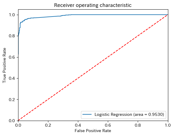
9.7.5.3.4. ROC Curve

from sklearn.metrics import roc_auc_score
from sklearn.metrics import roc_curve
logit_roc_auc = roc_auc_score(y_test, y_pred)
fpr, tpr, thresholds = roc_curve(y_test, clf.predict_proba(X_test)[:,1])
plt.figure()
plt.plot(fpr, tpr, label='Logistic Regression (area = %0.4f)' % logit_roc_auc)
plt.plot([0, 1], [0, 1],'r--')
plt.xlim([0.0, 1.0])
plt.ylim([0.0, 1.05])
plt.xlabel('False Positive Rate')
plt.ylabel('True Positive Rate')
plt.title('Receiver operating characteristic')
plt.legend(loc="lower right")
plt.show()

9.7.5.4. 2. Naive Bayse (Support Vector Machines)

from sklearn.naive_bayes import BernoulliNB
nb = BernoulliNB().fit(X_train, y_train)
y_pred = nb.predict(X_test)

9.7.5.4.1. Modelの精度

from sklearn.metrics import classification_report
print(classification_report(y_test, y_pred, target_names=cat.categories))

              precision    recall  f1-score   support

   AbeShinzo       0.92      0.96      0.94       486
hashimoto_lo       0.97      0.93      0.95       575

    accuracy                           0.94      1061
   macro avg       0.94      0.95      0.94      1061
weighted avg       0.95      0.94      0.94      1061

9.7.5.4.2. Confusion Matirx

print(metrics.confusion_matrix(y_test, y_pred))

[[467  19]
 [ 40 535]]

pd.DataFrame(metrics.confusion_matrix(y_test, y_pred), columns = cat.categories,
             index = cat.categories)

	AbeShinzo	hashimoto_lo
AbeShinzo	467	19
hashimoto_lo	40	535

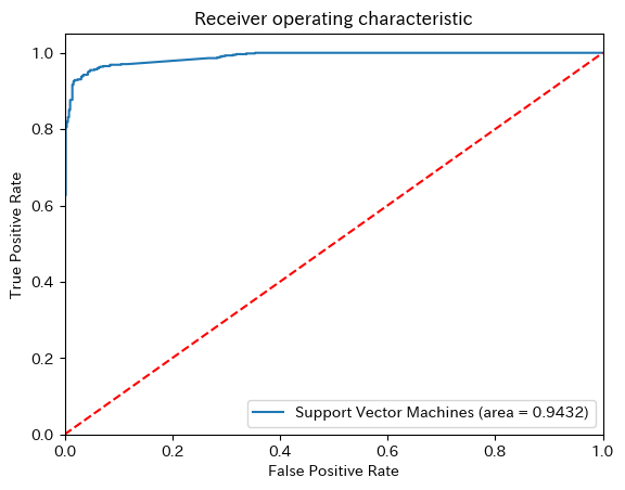
9.7.5.4.3. ROC Curve

logit_roc_auc = roc_auc_score(y_test, y_pred)
fpr, tpr, thresholds = roc_curve(y_test, clf.predict_proba(X_test)[:,1])
plt.figure()
plt.plot(fpr, tpr, label='Support Vector Machines (area = %0.4f)' % logit_roc_auc)
plt.plot([0, 1], [0, 1],'r--')
plt.xlim([0.0, 1.0])
plt.ylim([0.0, 1.05])
plt.xlabel('False Positive Rate')
plt.ylabel('True Positive Rate')
plt.title('Receiver operating characteristic')
plt.legend(loc="lower right")
plt.show()

9.7.5.5. 3. SVM (Support Vector Machines)

svm = svm.SVC(random_state=0).fit(X_train, y_train)
y_pred = svm.predict(X_test)

9.7.5.5.1. Modelの精度

print(classification_report(y_test, y_pred, target_names=cat.categories))

              precision    recall  f1-score   support

   AbeShinzo       0.91      0.96      0.94       486
hashimoto_lo       0.97      0.92      0.94       575

    accuracy                           0.94      1061
   macro avg       0.94      0.94      0.94      1061
weighted avg       0.94      0.94      0.94      1061

9.7.5.5.2. Confusion Matirx

print(metrics.confusion_matrix(y_test, y_pred))

[[468  18]
 [ 44 531]]

pd.DataFrame(metrics.confusion_matrix(y_test, y_pred), columns = cat.categories,
             index = cat.categories)

	AbeShinzo	hashimoto_lo
AbeShinzo	468	18
hashimoto_lo	44	531

9.7.5.5.3. ROC Curve

logit_roc_auc = roc_auc_score(y_test, y_pred)
fpr, tpr, thresholds = roc_curve(y_test, clf.predict_proba(X_test)[:,1])
plt.figure()
plt.plot(fpr, tpr, label='Support Vector Machines (area = %0.4f)' % logit_roc_auc)
plt.plot([0, 1], [0, 1],'r--')
plt.xlim([0.0, 1.0])
plt.ylim([0.0, 1.05])
plt.xlabel('False Positive Rate')
plt.ylabel('True Positive Rate')
plt.title('Receiver operating characteristic')
plt.legend(loc="lower right")
plt.show()

9.7.5.6. 4. Random Forest

rf = RandomForestClassifier(random_state=0).fit(X_train, y_train)
y_pred = rf.predict(X_test)

9.7.5.6.1. Modelの精度

from sklearn.metrics import classification_report
print(classification_report(y_test, y_pred, target_names=cat.categories))

              precision    recall  f1-score   support

   AbeShinzo       0.93      0.94      0.93       486
hashimoto_lo       0.95      0.94      0.94       575

    accuracy                           0.94      1061
   macro avg       0.94      0.94      0.94      1061
weighted avg       0.94      0.94      0.94      1061

9.7.5.6.2. Confusion Matirx

from sklearn import metrics
print(metrics.confusion_matrix(y_test, y_pred))

[[455  31]
 [ 35 540]]

pd.DataFrame(metrics.confusion_matrix(y_test, y_pred), columns = cat.categories,
             index = cat.categories)

	AbeShinzo	hashimoto_lo
AbeShinzo	455	31
hashimoto_lo	35	540

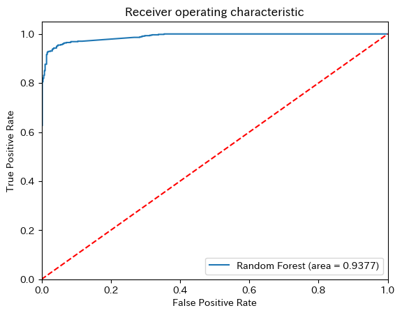
9.7.5.6.3. ROC Curve

logit_roc_auc = roc_auc_score(y_test, y_pred)
fpr, tpr, thresholds = roc_curve(y_test, clf.predict_proba(X_test)[:,1])
plt.figure()
plt.plot(fpr, tpr, label='Random Forest (area = %0.4f)' % logit_roc_auc)
plt.plot([0, 1], [0, 1],'r--')
plt.xlim([0.0, 1.0])
plt.ylim([0.0, 1.05])
plt.xlabel('False Positive Rate')
plt.ylabel('True Positive Rate')
plt.title('Receiver operating characteristic')
plt.legend(loc="lower right")
plt.show()

9.7.5.6.4. 5. Neural Netowrk

一般的にはsklearnではなくて、TensorflowやKerasを用いて実装することが多いのですが、ここではsklearnで実行します。

nn = MLPClassifier(random_state=0, max_iter=300, hidden_layer_sizes= 50).fit(X_train, y_train)
y_pred = nn.predict(X_test)

9.7.5.6.5. Modelの精度

print(classification_report(y_test, y_pred, target_names=cat.categories))

              precision    recall  f1-score   support

   AbeShinzo       0.94      0.98      0.96       486
hashimoto_lo       0.98      0.95      0.96       575

    accuracy                           0.96      1061
   macro avg       0.96      0.96      0.96      1061
weighted avg       0.96      0.96      0.96      1061

9.7.5.6.6. Confusion Matirx

print(metrics.confusion_matrix(y_test, y_pred))

[[474  12]
 [ 30 545]]

pd.DataFrame(metrics.confusion_matrix(y_test, y_pred), columns = cat.categories,
             index = cat.categories)

	AbeShinzo	hashimoto_lo
AbeShinzo	474	12
hashimoto_lo	30	545

9.7.5.6.7. ROC Curve

logit_roc_auc = roc_auc_score(y_test, y_pred)
fpr, tpr, thresholds = roc_curve(y_test, clf.predict_proba(X_test)[:,1])
plt.figure()
plt.plot(fpr, tpr, label='Neural Network (area = %0.4f)' % logit_roc_auc)
plt.plot([0, 1], [0, 1],'r--')
plt.xlim([0.0, 1.0])
plt.ylim([0.0, 1.05])
plt.xlabel('False Positive Rate')
plt.ylabel('True Positive Rate')
plt.title('Receiver operating characteristic')
plt.legend(loc="lower right")
plt.show()

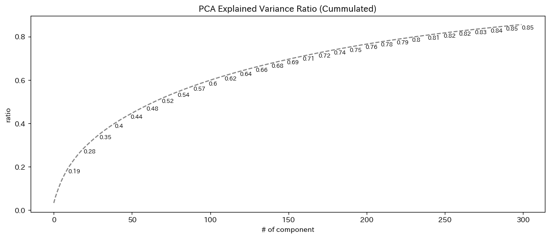
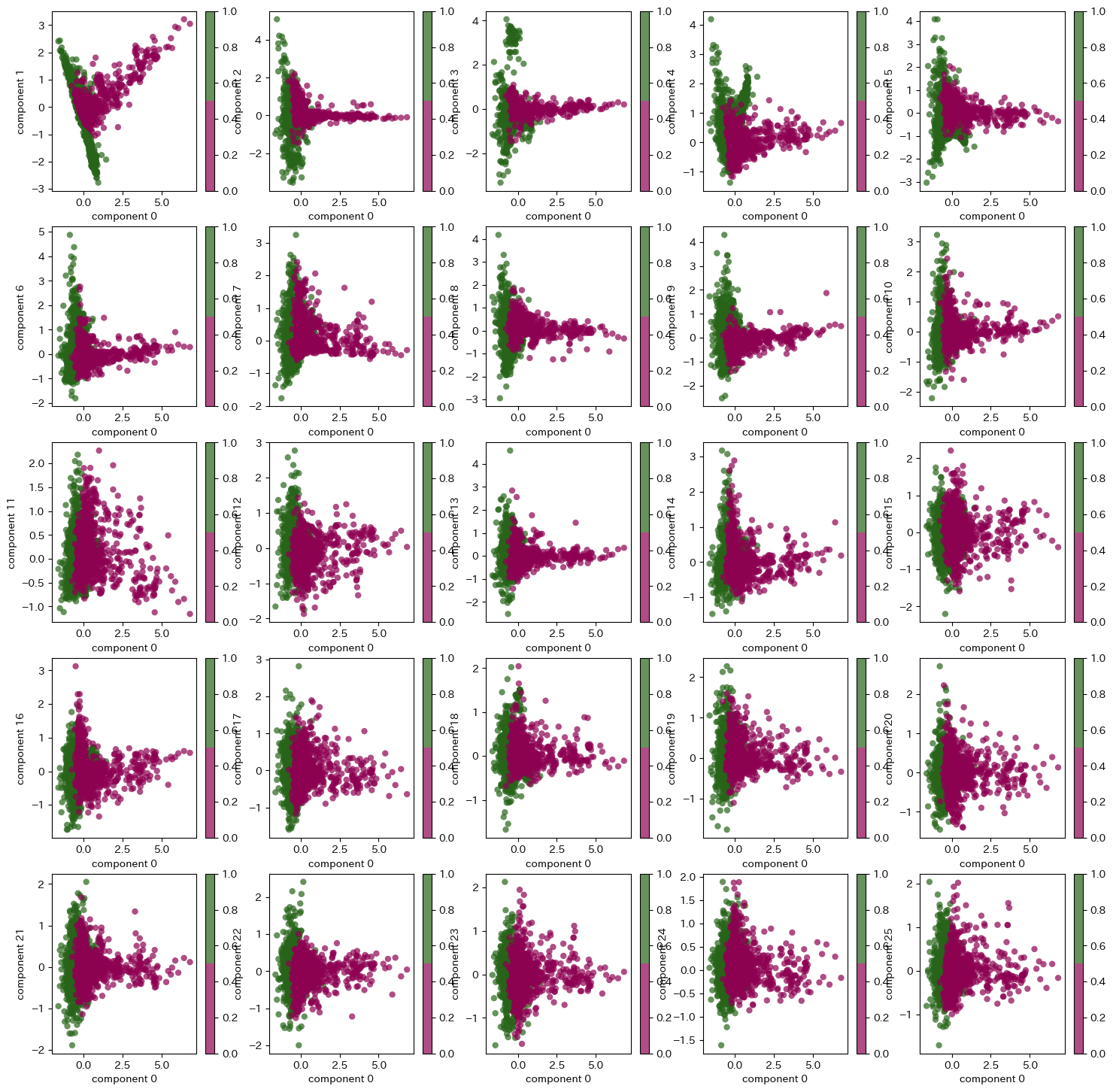
9.7.6. PCAによる次元圧縮

X_train, X_test, y_train, y_test = train_test_split(X, y, test_size=0.25, random_state=42)

X_train.shape

(3183, 690)

# 標準化
from sklearn.preprocessing import StandardScaler
scaler = StandardScaler()
# 平均と分散を計算
scaler.fit(X_train)
X_train_s = scaler.transform(X_train)
X_test_s  = scaler.transform(X_test)

pca = PCA(n_components=300)
pca.fit(X)
Xpca = pca.transform(X)
X_train = pca.transform(X_train_s)
X_test = pca.transform(X_test_s)

/opt/anaconda3/lib/python3.11/site-packages/sklearn/base.py:439: UserWarning: X does not have valid feature names, but PCA was fitted with feature names
  warnings.warn(
/opt/anaconda3/lib/python3.11/site-packages/sklearn/base.py:439: UserWarning: X does not have valid feature names, but PCA was fitted with feature names
  warnings.warn(

plt.figure(figsize=(13,5))
plt.plot(pca.explained_variance_ratio_.cumsum(),'--', color = 'grey')
for i, ratio in enumerate(pca.explained_variance_ratio_.cumsum()):
    if (i+1) % 10 ==0:
        plt.text(i, ratio-0.02, round(ratio,2), fontsize=8)
plt.title('PCA Explained Variance Ratio (Cummulated)')
plt.xlabel('# of component')
plt.ylabel('ratio')
plt.show()

fig, ax = plt.subplots(5,5, figsize = (18,18))
for i, combination in enumerate(list(itertools.combinations(range(len(pca.components_)), 2))[:25]):
    c = i // 5
    i = i - 5*c
    s1 = ax[c, i].scatter(Xpca[:, combination[0]], Xpca[:, combination[1]],
                c=cat.codes, 
                edgecolor='none', alpha=0.7,
                cmap=plt.cm.get_cmap('PiYG', 2))
    ax[c, i].set_xlabel('component {}'.format(combination[0]))
    ax[c, i].set_ylabel('component {}'.format(combination[1]))
    plt.colorbar(s1, ax = ax[c, i])
plt.show()

/var/folders/z5/0lnyp_m54dqc1xkz22ncbj2h0000gn/T/ipykernel_33116/2017848199.py:8: MatplotlibDeprecationWarning: The get_cmap function was deprecated in Matplotlib 3.7 and will be removed two minor releases later. Use ``matplotlib.colormaps[name]`` or ``matplotlib.colormaps.get_cmap(obj)`` instead.
  cmap=plt.cm.get_cmap('PiYG', 2))

# logistic regression
lg = LogisticRegression(random_state=0).fit(X_train, y_train)
lg_y_pred = lg.predict(X_test)
# Naive Bayse
nb = BernoulliNB().fit(X_train, y_train)
nb_y_pred = nb.predict(X_test)
# Random Forest
rf = RandomForestClassifier(random_state=0).fit(X_train, y_train)
rf_y_pred = rf.predict(X_test)
# Neural Network
nf = MLPClassifier(random_state=0).fit(X_train, y_train)
nf_y_pred = nf.predict(X_test)

print(metrics.accuracy_score(y_test, lg_y_pred))
print(metrics.accuracy_score(y_test, nb_y_pred))
print(metrics.accuracy_score(y_test, rf_y_pred))
print(metrics.accuracy_score(y_test, nf_y_pred))

0.9387370405278039
0.7577756833176249
0.9302544769085768
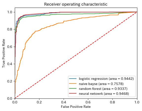
0.943449575871819

plt.figure()
names = ['logistic regression','naive bayse', 'random forest', 'neural netowrk']
for i, tmp in enumerate(zip([lg_y_pred, nb_y_pred, rf_y_pred, nf_y_pred],[lg,nb,rf,nf])):
    roc_auc = roc_auc_score(y_test, tmp[0])
    fpr, tpr, thresholds = roc_curve(y_test, tmp[1].predict_proba(X_test)[:,1])
    plt.plot(fpr, tpr, label='{} (area = {})'.format(names[i], round(roc_auc, 4)))
plt.plot([0, 1], [0, 1],'r--')
plt.xlim([0.0, 1.0])
plt.ylim([0.0, 1.05])
plt.xlabel('False Positive Rate')
plt.ylabel('True Positive Rate')
plt.title('Receiver operating characteristic')
plt.legend(loc="lower right")
plt.show()

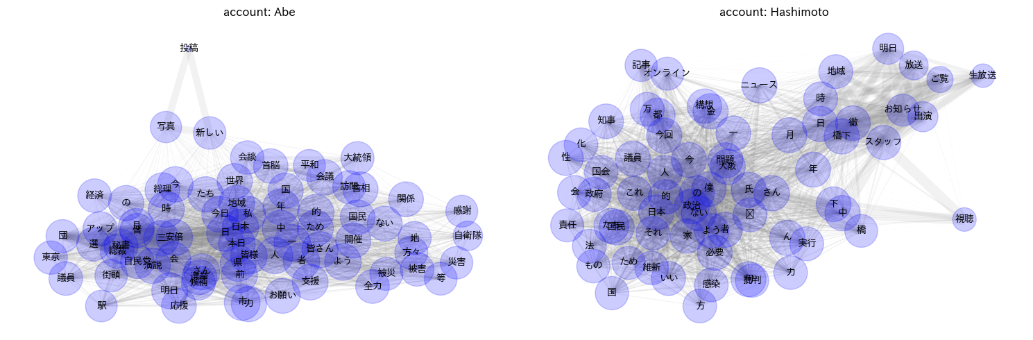
9.7.7. どのようなトピックがあるか単語共起ネットワークを描く

import networkx as nx

アカウントごとに、単語の共起関係を示す共起行列を作ります

df_hashimoto = df[df['user_screen_name']=='hashimoto_lo']
df_abe = df[df['user_screen_name']=='AbeShinzo']

count_model = CountVectorizer(analyzer=tokenize, ngram_range=(1,1), min_df=0.03, max_df=.95) 
X_a = count_model.fit_transform(df_abe['standarized_text'])
X_a[X_a > 0] = 1 
Xc_a = (X_a.T * X_a)
Xc_a.setdiag(0) 
wordword_a = pd.DataFrame(Xc_a.todense(), index = count_model.get_feature_names_out(),columns = count_model.get_feature_names_out())
wordword_a.shape

(74, 74)

# `min_df`で指定した値より少ない出現回数の単語は除外します。
# `max_df`で指定した値より多い出現回数の単語は除外します。[0, 1]の間の値で割合での指定もできます。
count_model = CountVectorizer(analyzer=tokenize, ngram_range=(1,1), min_df=0.04, max_df=.95) 
X_h = count_model.fit_transform(df_hashimoto['standarized_text'])
X_h[X_h > 0] = 1 
Xc_h = (X_h.T * X_h)
Xc_h.setdiag(0) 
wordword_h = pd.DataFrame(Xc_h.todense(), index = count_model.get_feature_names_out(),columns = count_model.get_feature_names_out())
wordword_h.shape

(69, 69)

# create network
G_h = nx.from_pandas_adjacency(wordword_h)
G_a = nx.from_pandas_adjacency(wordword_a)

fig, axs = plt.subplots(1, 2, figsize=(15, 5))
for i in range(2):
    ax = axs[i]
    G = [G_a, G_h][i]
    # Position nodes using Fruchterman-Reingold force-directed algorithm.
    # https://networkx.org/documentation/stable/reference/generated/networkx.drawing.layout.spring_layout.html
    pos = nx.spring_layout(G, seed=999)
    d = dict(G.degree)
    weights = [G[u][v]['weight']*0.1 for u,v in G.edges()]
    nx.draw_networkx_nodes(G, pos, ax=ax, node_color='blue', node_size=[v * 20 for v in d.values()], alpha = 0.2)
    nx.draw_networkx_edges(G, pos, ax=ax, alpha=0.1, width=list(weights), edge_color = 'grey')
    nx.draw_networkx_labels(G, pos, ax=ax, font_family='IPAexGothic', font_size=10)
    ax.set_title('account: {}'.format(['Abe', 'Hashimoto'][i]))
    ax.axis('off')
plt.tight_layout()
plt.show()

/opt/anaconda3/lib/python3.11/site-packages/IPython/core/pylabtools.py:152: UserWarning: Glyph 10145 (\N{BLACK RIGHTWARDS ARROW}) missing from current font.
  fig.canvas.print_figure(bytes_io, **kw)

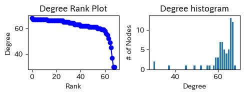
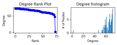
for c, G in enumerate([G_a, G_h]):
    print(['Abe','Hashimoto'][c])
    degree_sequence = sorted((d for n, d in G.degree()), reverse=True)
    dmax = max(degree_sequence)
    fig, axs = plt.subplots(1, 2, figsize=(5, 2))
    ax = axs[0]
    ax.plot(degree_sequence, "b-", marker="o")
    ax.set_title("Degree Rank Plot")
    ax.set_ylabel("Degree")
    ax.set_xlabel("Rank")

    ax = axs[1]
    ax.bar(*np.unique(degree_sequence, return_counts=True))
    ax.set_title("Degree histogram")
    ax.set_xlabel("Degree")
    ax.set_ylabel("# of Nodes")
    plt.tight_layout()
    plt.show()

Abe

Hashimoto