9.2. Yahoo! FINANCEのデータを用いた可視化の演習#
ここからは米国のYahoo! FINANCEの株価データを用いて相関関係の可視化を行います。
今日現在までの直近1年間のtech_stockおよび日系企業の株価データを用います。
Pythonで
Yahoo! FINANCEのデータを集めるパッケージyfinanceを用います。
Warning
ここで用いるパッケージyfinanceはYahooが公開しているAPIを利用したオープンソースのツールであり、研究・教育目的での利用を想定しています。 ダウンロードした実際のデータを使用する権利の詳細については、ヤフーの利用規約を参照する必要があります(Yahoo Developer API Terms of Use; Yahoo Terms of Service; Yahoo Terms)。
ここで紹介する企業以外を試す場合は、Yahoo! FINANCEのページで企業の銘柄コードを確認して置き換えてください。
Warning
必要なパッケージをインストールします。すでに、requirements.txtを用いてパッケージ類をインストールしている場合は、そのまま次のセルに進んでください。
まだの場合は、こちらのページを用いてパッケージ類をインストールしてください。もしくは、以下の方法をお試しください。
WinodwsのかたはWindowsのメニューから
Anaconda Propmtを、Macの方はTerminalを起動させ、conda install gitを入力してエンターを押してください。しばらくするとProceed ([y]/n)?と表示されるのでyを入力してエンターを押して続行してください。pip install git+https://github.com/pydata/pandas-datareaderを入力しエンターを押して、pandas-datareaderのインストールを実行します。Terminal上で、
pip install yfinance --upgrade --no-cache-dirを入力しエンターを押してyfinanceのインストールを実行します。
from datetime import datetime
import os
import pandas as pd
from pandas_datareader import data as pdr
import matplotlib.pyplot as plt
import numpy as np
import yfinance as yf
end = datetime.now()
start =  datetime(end.year-1, end.month, end.day)

yf.pdr_override()

tech_stock = ['GOOG', 'AAPL', 'META', 'AMZN', 'NFLX', 'TSLA']

for company in tech_stock:
    globals()[company] = pdr.get_data_yahoo(tickers=company, start=start, end=end)
[*********************100%%**********************] 1 of 1 completed
[*********************100%%**********************] 1 of 1 completed
[*********************100%%**********************] 1 of 1 completed
[*********************100%%**********************] 1 of 1 completed
[*********************100%%**********************] 1 of 1 completed
[*********************100%%**********************] 1 of 1 completed
Open:始値
High:高値
Low:安値
Close:終値
Volume:出来高(1日に取引が成立した株の数)
Adj Close:調整後終値
GOOG.describe()
| Open | High | Low | Close | Adj Close | Volume | |
|---|---|---|---|---|---|---|
| count | 250.000000 | 250.000000 | 250.000000 | 250.000000 | 250.000000 | 2.500000e+02 |
| mean | 164.983688 | 166.702312 | 163.429972 | 165.065400 | 164.667500 | 1.975175e+07 |
| std | 15.350093 | 15.567643 | 15.179647 | 15.360177 | 15.432170 | 8.323973e+06 |
| min | 132.740005 | 134.020004 | 131.550003 | 132.559998 | 132.085388 | 6.809800e+06 |
| 25% | 152.992496 | 154.889996 | 151.707497 | 153.197502 | 152.649017 | 1.456728e+07 |
| 50% | 166.119995 | 167.770004 | 164.775002 | 166.139999 | 165.792549 | 1.752165e+07 |
| 75% | 175.824005 | 178.022495 | 174.869995 | 176.419998 | 175.998856 | 2.166620e+07 |
| max | 198.529999 | 202.880005 | 196.690002 | 198.160004 | 198.160004 | 5.972800e+07 |
GOOG.info()
<class 'pandas.core.frame.DataFrame'>
DatetimeIndex: 250 entries, 2024-01-02 to 2024-12-27
Data columns (total 6 columns):
 #   Column     Non-Null Count  Dtype
---  ------     --------------  -----
 0   Open       250 non-null    float64
 1   High       250 non-null    float64
 2   Low        250 non-null    float64
 3   Close      250 non-null    float64
 4   Adj Close  250 non-null    float64
 5   Volume     250 non-null    int64
dtypes: float64(5), int64(1)
memory usage: 13.7 KB
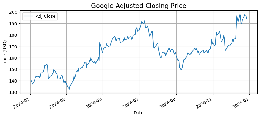
# Google の調整済終値のプロット
GOOG['Adj Close'].plot(legend=True, figsize=(10,4))
plt.title("Google Adjusted Closing Price", fontsize=15)
plt.ylabel('price (USD)')
plt.grid()
plt.show()
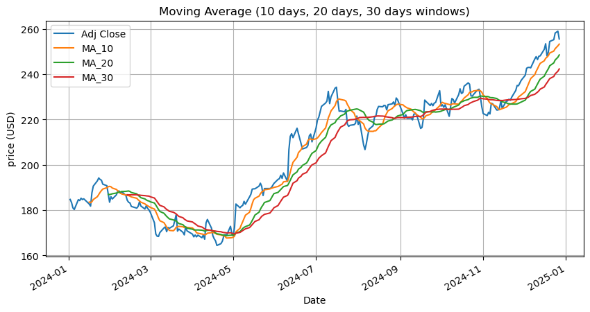
9.2.1. 移動平均(Moving Average)#
時系列データで一定区間ごとの平均値を区間をずらしながら求めたもの
ma_day = [10, 20, 30] # 10日、20日、50日の移動平均の値を持つ新しいcolumn(MA_10, MA_20, MA_50)を作ります
for ma in ma_day:
    for company in [GOOG, AAPL, META, NFLX, AMZN]:
        company['MA_{}'.format(ma)] = company['Adj Close'].rolling(ma).mean() #rolling(日数).mean()で日数の移動平均を求めます
AAPL.head(3)
| Open | High | Low | Close | Adj Close | Volume | MA_10 | MA_20 | MA_30 | |
|---|---|---|---|---|---|---|---|---|---|
| Date | |||||||||
| 2024-01-02 | 187.149994 | 188.440002 | 183.889999 | 185.639999 | 184.734985 | 82488700 | NaN | NaN | NaN |
| 2024-01-03 | 184.220001 | 185.880005 | 183.429993 | 184.250000 | 183.351761 | 58414500 | NaN | NaN | NaN |
| 2024-01-04 | 182.149994 | 183.089996 | 180.880005 | 181.910004 | 181.023178 | 71983600 | NaN | NaN | NaN |
AAPL[['Adj Close','MA_10', 'MA_20','MA_30']].plot(subplots=False, figsize=(10,5))
plt.title('Moving Average (10 days, 20 days, 30 days windows)')
plt.ylabel('price (USD)')
plt.grid()
plt.show()
9.2.2. 参考: 株価の前日からのパーセント変化を求めます#
for company in [GOOG, AAPL, META, AMZN, NFLX,TSLA]:
    company['returns'] = company['Adj Close'].pct_change()
colors = ['orange','black','blue','red','yellow','green']
i=0
plt.figure(figsize=(8,5))
for company in [GOOG, AAPL, META, AMZN, NFLX, TSLA]:
    plt.hist(company['returns'].dropna(),bins=100,color=colors[i],alpha = 0.2, label=tech_stock[i])
    i += 1
plt.legend()
plt.xlabel('Percentage change')
plt.ylabel('Frequency')
plt.grid(axis='x')
plt.show()
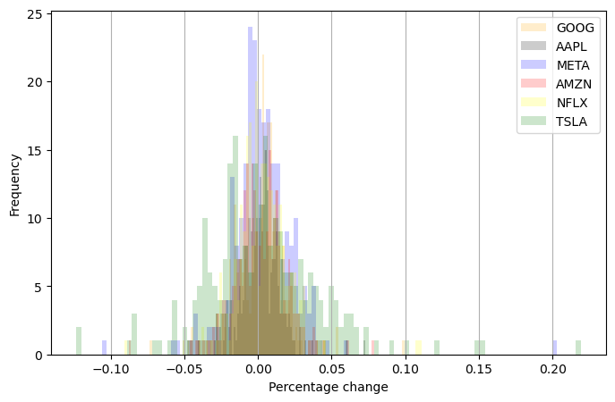
ヒストグラムで6社の変化率を上のように示すと、6社とも多くの日で前日からの変化率は??%以内。
6社の終値を格納したDataFrameを作成します
tech_stock_close = pd.DataFrame({'GOOG':GOOG['Adj Close'],
                           'AAPL':AAPL['Adj Close'],
                           'META': META['Adj Close'],
                           'AMZN': AMZN['Adj Close'],
                           'NFLX': NFLX['Adj Close'],
                           'TSLA': TSLA['Adj Close']})
tech_stock_close.describe()
| GOOG | AAPL | META | AMZN | NFLX | TSLA | |
|---|---|---|---|---|---|---|
| count | 250.000000 | 250.000000 | 250.000000 | 250.000000 | 250.000000 | 250.000000 |
| mean | 164.667500 | 206.413754 | 507.638002 | 184.342960 | 669.705240 | 229.174880 |
| std | 15.432170 | 25.505410 | 62.309650 | 17.199507 | 108.823840 | 69.406924 |
| min | 132.085388 | 164.405121 | 343.159119 | 144.570007 | 468.500000 | 142.050003 |
| 25% | 152.649017 | 183.385338 | 474.307808 | 175.360004 | 608.745010 | 179.995003 |
| 50% | 165.792549 | 213.687302 | 503.563019 | 183.260002 | 647.629974 | 210.630005 |
| 75% | 175.998856 | 227.032825 | 562.201508 | 189.395000 | 706.632492 | 248.372498 |
| max | 198.160004 | 259.019989 | 632.170044 | 232.929993 | 936.559998 | 479.859985 |
tech_stock_close.info()
<class 'pandas.core.frame.DataFrame'>
DatetimeIndex: 250 entries, 2024-01-02 to 2024-12-27
Data columns (total 6 columns):
 #   Column  Non-Null Count  Dtype
---  ------  --------------  -----
 0   GOOG    250 non-null    float64
 1   AAPL    250 non-null    float64
 2   META    250 non-null    float64
 3   AMZN    250 non-null    float64
 4   NFLX    250 non-null    float64
 5   TSLA    250 non-null    float64
dtypes: float64(6)
memory usage: 13.7 KB
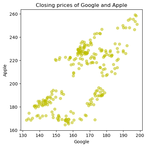
9.2.2.1. GoogleとApple#
GoogleとApple の直近1年間の株価終値の相関係数を求めます。
tech_stock_close['GOOG'].corr(tech_stock_close['AAPL'])
0.6755733160023757
GoogleとApple の直近1年間の株価終値の相関行列を示します。
tech_stock_close[['GOOG','AAPL']].corr()
| GOOG | AAPL | |
|---|---|---|
| GOOG | 1.000000 | 0.675573 |
| AAPL | 0.675573 | 1.000000 |
GoogleとApple の直近1年間の株価終値の散布図を示します。
plt.figure(figsize=(5,5))
plt.scatter(tech_stock_close['GOOG'],tech_stock_close['AAPL'],color ='y',alpha=0.5)
plt.xlabel('Google')
plt.ylabel('Apple')
plt.title("Closing prices of Google and Apple")
plt.show()
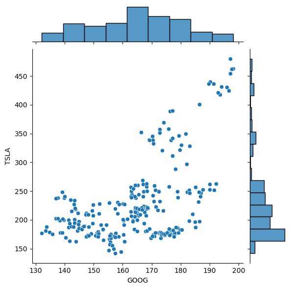
9.2.2.2. ヒストグラムと散布図を1つの図中に示す方法#
import seaborn as sns

sns.jointplot(data=tech_stock_close, x='GOOG', y='TSLA')
plt.show()
/opt/anaconda3/lib/python3.11/site-packages/seaborn/_oldcore.py:1119: FutureWarning: use_inf_as_na option is deprecated and will be removed in a future version. Convert inf values to NaN before operating instead.
  with pd.option_context('mode.use_inf_as_na', True):
/opt/anaconda3/lib/python3.11/site-packages/seaborn/_oldcore.py:1119: FutureWarning: use_inf_as_na option is deprecated and will be removed in a future version. Convert inf values to NaN before operating instead.
  with pd.option_context('mode.use_inf_as_na', True):
sns.pairplot(tech_stock_close, plot_kws=dict(color = 'b', edgecolor='b', alpha = 0.2))
plt.show()
/opt/anaconda3/lib/python3.11/site-packages/seaborn/_oldcore.py:1119: FutureWarning: use_inf_as_na option is deprecated and will be removed in a future version. Convert inf values to NaN before operating instead.
  with pd.option_context('mode.use_inf_as_na', True):
/opt/anaconda3/lib/python3.11/site-packages/seaborn/_oldcore.py:1119: FutureWarning: use_inf_as_na option is deprecated and will be removed in a future version. Convert inf values to NaN before operating instead.
  with pd.option_context('mode.use_inf_as_na', True):
/opt/anaconda3/lib/python3.11/site-packages/seaborn/_oldcore.py:1119: FutureWarning: use_inf_as_na option is deprecated and will be removed in a future version. Convert inf values to NaN before operating instead.
  with pd.option_context('mode.use_inf_as_na', True):
/opt/anaconda3/lib/python3.11/site-packages/seaborn/_oldcore.py:1119: FutureWarning: use_inf_as_na option is deprecated and will be removed in a future version. Convert inf values to NaN before operating instead.
  with pd.option_context('mode.use_inf_as_na', True):
/opt/anaconda3/lib/python3.11/site-packages/seaborn/_oldcore.py:1119: FutureWarning: use_inf_as_na option is deprecated and will be removed in a future version. Convert inf values to NaN before operating instead.
  with pd.option_context('mode.use_inf_as_na', True):
/opt/anaconda3/lib/python3.11/site-packages/seaborn/_oldcore.py:1119: FutureWarning: use_inf_as_na option is deprecated and will be removed in a future version. Convert inf values to NaN before operating instead.
  with pd.option_context('mode.use_inf_as_na', True):
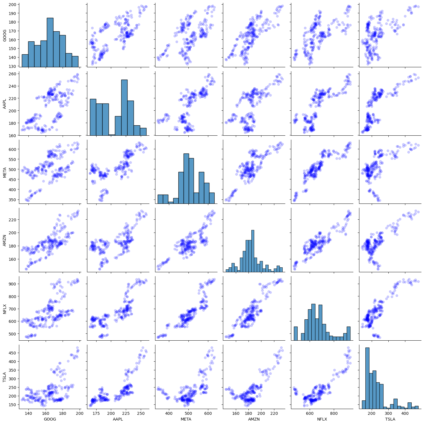
6社の相関行列を示します。
tech_stock_close.corr()
| GOOG | AAPL | META | AMZN | NFLX | TSLA | |
|---|---|---|---|---|---|---|
| GOOG | 1.000000 | 0.675573 | 0.545528 | 0.762449 | 0.661126 | 0.542634 |
| AAPL | 0.675573 | 1.000000 | 0.699146 | 0.642521 | 0.795830 | 0.765408 |
| META | 0.545528 | 0.699146 | 1.000000 | 0.823320 | 0.888165 | 0.606519 |
| AMZN | 0.762449 | 0.642521 | 0.823320 | 1.000000 | 0.897526 | 0.750186 |
| NFLX | 0.661126 | 0.795830 | 0.888165 | 0.897526 | 1.000000 | 0.825915 |
| TSLA | 0.542634 | 0.765408 | 0.606519 | 0.750186 | 0.825915 | 1.000000 |
9.2.2.2.1. 参考#
続いて日本の自動車メーカーのToyota Motor CorporationとHonda Motor Co., Ltd.の直近1年の株価も収集します。
end = datetime.now()
start =  datetime(end.year-1, end.month, end.day)

yf.pdr_override()

vehicles = ['TM', 'HMC'] # TM : Toyota Motor Corporation, HMC: Honda Motor Co., Ltd.
for company in vehicles:
    globals()[company] = pdr.get_data_yahoo(tickers=company, start=start, end=end)
[*********************100%%**********************] 1 of 1 completed
[*********************100%%**********************] 1 of 1 completed
print(TM.info(), HMC.info())
<class 'pandas.core.frame.DataFrame'>
DatetimeIndex: 250 entries, 2024-01-02 to 2024-12-27
Data columns (total 6 columns):
 #   Column     Non-Null Count  Dtype
---  ------     --------------  -----
 0   Open       250 non-null    float64
 1   High       250 non-null    float64
 2   Low        250 non-null    float64
 3   Close      250 non-null    float64
 4   Adj Close  250 non-null    float64
 5   Volume     250 non-null    int64
dtypes: float64(5), int64(1)
memory usage: 13.7 KB
None None
tm_hmc = pd.DataFrame({'TM':TM['Adj Close'],'HMC':HMC['Adj Close']})
tech_stock_th = pd.concat([tech_stock_close, tm_hmc], axis=1)
tech_stock_th.sample(4)
| GOOG | AAPL | META | AMZN | NFLX | TSLA | TM | HMC | |
|---|---|---|---|---|---|---|---|---|
| Date | ||||||||
| 2024-04-22 | 157.384491 | 165.242081 | 480.405975 | 177.229996 | 554.599976 | 142.050003 | 230.300003 | 34.549999 |
| 2024-09-09 | 149.370529 | 220.667221 | 503.902435 | 175.399994 | 675.419983 | 216.270004 | 176.080002 | 31.530001 |
| 2024-02-26 | 138.253235 | 180.506866 | 480.415955 | 174.729996 | 587.650024 | 199.399994 | 238.130005 | 35.660000 |
| 2024-05-13 | 170.288132 | 185.860138 | 466.723724 | 186.570007 | 616.590027 | 171.889999 | 215.639999 | 33.790001 |
# データを保存
os.makedirs('./data', exist_ok=True)
tech_stock_close.to_csv('./data/tech_stock_close.csv')
tech_stock_close.to_pickle('./data/tech_stock_close.pkl')
tech_stock4社と自動車メーカー2社の相関行列を示します。
tech_stock_th.corr()
| GOOG | AAPL | META | AMZN | NFLX | TSLA | TM | HMC | |
|---|---|---|---|---|---|---|---|---|
| GOOG | 1.000000 | 0.675573 | 0.545528 | 0.762449 | 0.661126 | 0.542634 | -0.413725 | -0.583584 |
| AAPL | 0.675573 | 1.000000 | 0.699146 | 0.642521 | 0.795830 | 0.765408 | -0.838156 | -0.801696 |
| META | 0.545528 | 0.699146 | 1.000000 | 0.823320 | 0.888165 | 0.606519 | -0.429586 | -0.514580 |
| AMZN | 0.762449 | 0.642521 | 0.823320 | 1.000000 | 0.897526 | 0.750186 | -0.293303 | -0.603807 |
| NFLX | 0.661126 | 0.795830 | 0.888165 | 0.897526 | 1.000000 | 0.825915 | -0.550100 | -0.759890 |
| TSLA | 0.542634 | 0.765408 | 0.606519 | 0.750186 | 0.825915 | 1.000000 | -0.593509 | -0.846852 |
| TM | -0.413725 | -0.838156 | -0.429586 | -0.293303 | -0.550100 | -0.593509 | 1.000000 | 0.827525 |
| HMC | -0.583584 | -0.801696 | -0.514580 | -0.603807 | -0.759890 | -0.846852 | 0.827525 | 1.000000 |
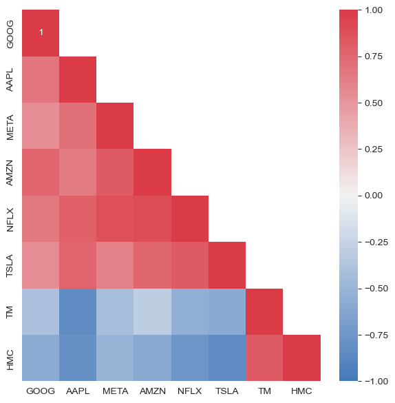
9.2.2.3. 参考: ヒートマップで相関関係を示す#
変数が多い場合視覚的にわかりやすい
def CorrMtx(df, dropDuplicates = True):

    if dropDuplicates:
        mask = np.zeros_like(df, dtype=bool)
        mask[np.triu_indices_from(mask,1)] = True

    sns.set_style(style = 'white')

    fig, ax = plt.subplots(figsize=(7, 7))

    cmap = sns.diverging_palette(250, 10, as_cmap=True)

    if dropDuplicates:
        sns.heatmap(df, mask=mask, vmin=-1, vmax=1,annot=True,cmap=cmap)
    else:
        sns.heatmap(df, vmin=-1, vmax=1,annot=True,cmap=cmap)


CorrMtx(tech_stock_th.corr(), dropDuplicates = True)
/opt/anaconda3/lib/python3.11/site-packages/seaborn/matrix.py:260: FutureWarning: Format strings passed to MaskedConstant are ignored, but in future may error or produce different behavior
  annotation = ("{:" + self.fmt + "}").format(val)
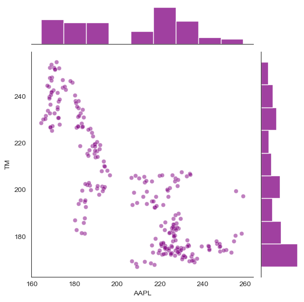
AppleとToyotaの散布図を示します。
sns.jointplot(x='AAPL', y='TM', data=tech_stock_th, color="purple", alpha = 0.5)
plt.show()
/opt/anaconda3/lib/python3.11/site-packages/seaborn/_oldcore.py:1119: FutureWarning: use_inf_as_na option is deprecated and will be removed in a future version. Convert inf values to NaN before operating instead.
  with pd.option_context('mode.use_inf_as_na', True):
/opt/anaconda3/lib/python3.11/site-packages/seaborn/_oldcore.py:1119: FutureWarning: use_inf_as_na option is deprecated and will be removed in a future version. Convert inf values to NaN before operating instead.
  with pd.option_context('mode.use_inf_as_na', True):
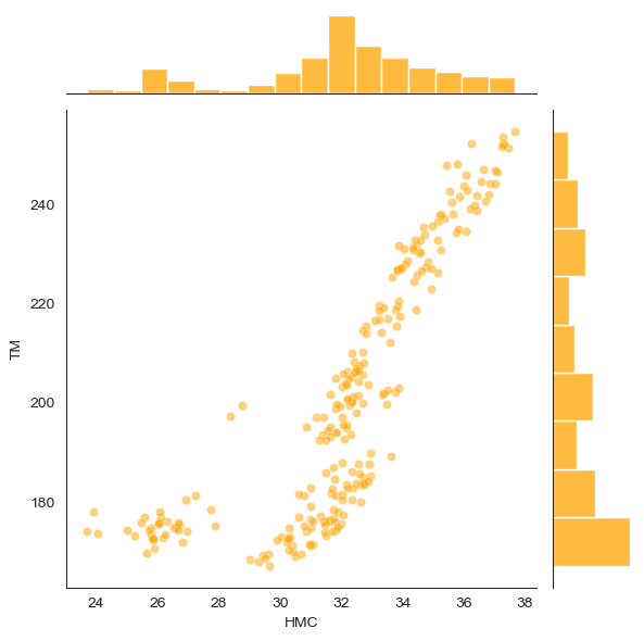
HondaとToyotaの散布図を示します。
sns.jointplot(x='HMC', y='TM', data=tech_stock_th, color="orange", alpha = 0.5)
plt.show()
/opt/anaconda3/lib/python3.11/site-packages/seaborn/_oldcore.py:1119: FutureWarning: use_inf_as_na option is deprecated and will be removed in a future version. Convert inf values to NaN before operating instead.
  with pd.option_context('mode.use_inf_as_na', True):
/opt/anaconda3/lib/python3.11/site-packages/seaborn/_oldcore.py:1119: FutureWarning: use_inf_as_na option is deprecated and will be removed in a future version. Convert inf values to NaN before operating instead.
  with pd.option_context('mode.use_inf_as_na', True):
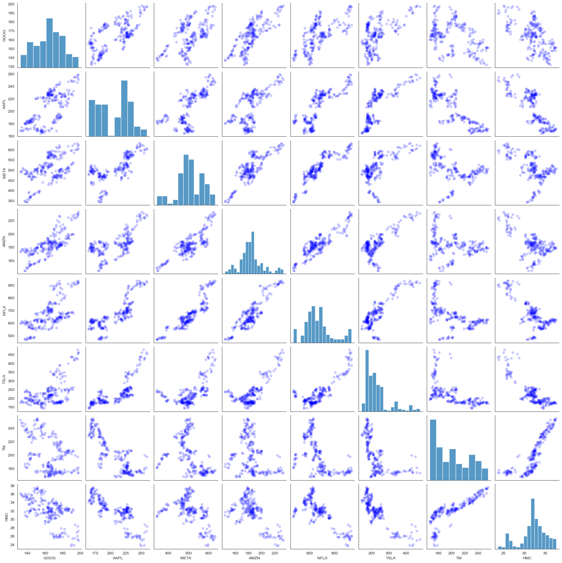
sns.pairplot(tech_stock_th, plot_kws=dict(color = 'blue', edgecolor='b', alpha = 0.2))
plt.show()
/opt/anaconda3/lib/python3.11/site-packages/seaborn/_oldcore.py:1119: FutureWarning: use_inf_as_na option is deprecated and will be removed in a future version. Convert inf values to NaN before operating instead.
  with pd.option_context('mode.use_inf_as_na', True):
/opt/anaconda3/lib/python3.11/site-packages/seaborn/_oldcore.py:1119: FutureWarning: use_inf_as_na option is deprecated and will be removed in a future version. Convert inf values to NaN before operating instead.
  with pd.option_context('mode.use_inf_as_na', True):
/opt/anaconda3/lib/python3.11/site-packages/seaborn/_oldcore.py:1119: FutureWarning: use_inf_as_na option is deprecated and will be removed in a future version. Convert inf values to NaN before operating instead.
  with pd.option_context('mode.use_inf_as_na', True):
/opt/anaconda3/lib/python3.11/site-packages/seaborn/_oldcore.py:1119: FutureWarning: use_inf_as_na option is deprecated and will be removed in a future version. Convert inf values to NaN before operating instead.
  with pd.option_context('mode.use_inf_as_na', True):
/opt/anaconda3/lib/python3.11/site-packages/seaborn/_oldcore.py:1119: FutureWarning: use_inf_as_na option is deprecated and will be removed in a future version. Convert inf values to NaN before operating instead.
  with pd.option_context('mode.use_inf_as_na', True):
/opt/anaconda3/lib/python3.11/site-packages/seaborn/_oldcore.py:1119: FutureWarning: use_inf_as_na option is deprecated and will be removed in a future version. Convert inf values to NaN before operating instead.
  with pd.option_context('mode.use_inf_as_na', True):
/opt/anaconda3/lib/python3.11/site-packages/seaborn/_oldcore.py:1119: FutureWarning: use_inf_as_na option is deprecated and will be removed in a future version. Convert inf values to NaN before operating instead.
  with pd.option_context('mode.use_inf_as_na', True):
/opt/anaconda3/lib/python3.11/site-packages/seaborn/_oldcore.py:1119: FutureWarning: use_inf_as_na option is deprecated and will be removed in a future version. Convert inf values to NaN before operating instead.
  with pd.option_context('mode.use_inf_as_na', True):
9.2.2.4. 参考:ロウソクチャートを描く#
Note
以下cufflinksというパッケージを用いて可視化を行います。
requirements.txtを用いて必要なパッケージをすでにインストールしている場合は、次のセルに進んでください。インストール方法はこちら必要なパッケージをご確認ください。
まだの場合などは、pip install cufflinksをターミナルで実行しcufflinksをインストールてから次のセルを実行してください。
import cufflinks as cf
cf.set_config_file(offline=True)

qf = cf.QuantFig(AAPL, legend='top', title = 'Apple Candle Chart')
qf.iplot()
qf = cf.QuantFig(AAPL, legend='top', title = 'Apple Candle Chart')
qf.add_volume()  # 出来高もプロット
qf.add_sma([10,50],width=2, color=['red', 'green'])  # 移動平均線もプロット
qf.iplot()
/opt/anaconda3/lib/python3.11/site-packages/cufflinks/quant_figure.py:1061: FutureWarning:

Series.__getitem__ treating keys as positions is deprecated. In a future version, integer keys will always be treated as labels (consistent with DataFrame behavior). To access a value by position, use `ser.iloc[pos]`