8.1. 機械学習#
機械学習は与えられたデータをよく表現できるようにモデルのパラメーターを調整し「学習」を行います。学習したモデルを用いることで、新たなデータに対する予測を行うことができます。
8.1.1. 機械学習の種類#
機械学習は次の3つに大別できます。このNotebookではこのうち教師あり学習と教師なし学習を扱います。
教師あり学習 (Supervised learning)
データの特徴(特徴量)に対して正解データ(正しい答え、ラベル、Ground Truth)がある場合は教師あり学習と呼ばれます。正解データを教師としてデータからラベルを予測できるように学習します。
分類 ラベルが離散値 (例:犬か猫かを予測する)
回帰 ラベルが連続値 (例:明日の株価を予測する)
教師なし学習 (Unsupervised learning)
ラベルがないデータのみからデータの構造や特徴・パターンなどをよく表すようなモデルをつくります。
クラスタリング
PCAなどの次元圧縮
強化学習 (Reinforcement learning)
ラベルはないですが報酬が与えられます。報酬を最大化するように学習する。
8.1.2. 機械学習のデータ#
学習データ(訓練データ、training data)
検証データ(テストデータ、testing data/validation data)
機械学習とは、データセットの特徴を学習し、別のデータセットに対してそれらの特徴をテストします。機械学習の一般的な方法は、データセットを2つに分割してアルゴリズムを評価することです。これらのセットのうちの1つを学習データ(training data)と呼び、そこから特徴を学習し、もう1つのセットを検証データ(testing data)と呼び、その上で学習した特徴をテストします。
ここではPythonのscikit-learnを用いて機械学習を動かしてみます。
8.1.3. 教師あり学習#
8.1.3.1. 分類問題#
まず、サンプルデータセットをダウンロードします。 3種類の花(iris)のがくへんの長さや・幅、花弁の長さや・幅が特徴量として与えられているデータです。 これらの特徴から、3種類のうちどの種類の花なのかを学習・予測します。
データで
0:
setosa1:
versicolor2:
virginica
を示します。
from sklearn import datasets
import pandas as pd
import numpy as np
from sklearn.linear_model import LogisticRegression, LinearRegression
from sklearn.model_selection import train_test_split
from sklearn.metrics import accuracy_score, confusion_matrix, classification_report, mean_squared_error
from sklearn import svm
from matplotlib import pyplot as plt
%matplotlib inline
data = datasets.load_iris()
df = pd.DataFrame(data.data, columns=data.feature_names).reset_index(drop=True)
target = pd.DataFrame(data.target, columns = ['species']).reset_index(drop=True)
df = df.merge(target, left_index=True, right_index=True, )
df.head()
| sepal length (cm) | sepal width (cm) | petal length (cm) | petal width (cm) | species | |
|---|---|---|---|---|---|
| 0 | 5.1 | 3.5 | 1.4 | 0.2 | 0 |
| 1 | 4.9 | 3.0 | 1.4 | 0.2 | 0 |
| 2 | 4.7 | 3.2 | 1.3 | 0.2 | 0 |
| 3 | 4.6 | 3.1 | 1.5 | 0.2 | 0 |
| 4 | 5.0 | 3.6 | 1.4 | 0.2 | 0 |
df.describe()
| sepal length (cm) | sepal width (cm) | petal length (cm) | petal width (cm) | species | |
|---|---|---|---|---|---|
| count | 150.000000 | 150.000000 | 150.000000 | 150.000000 | 150.000000 |
| mean | 5.843333 | 3.057333 | 3.758000 | 1.199333 | 1.000000 |
| std | 0.828066 | 0.435866 | 1.765298 | 0.762238 | 0.819232 |
| min | 4.300000 | 2.000000 | 1.000000 | 0.100000 | 0.000000 |
| 25% | 5.100000 | 2.800000 | 1.600000 | 0.300000 | 0.000000 |
| 50% | 5.800000 | 3.000000 | 4.350000 | 1.300000 | 1.000000 |
| 75% | 6.400000 | 3.300000 | 5.100000 | 1.800000 | 2.000000 |
| max | 7.900000 | 4.400000 | 6.900000 | 2.500000 | 2.000000 |
X = df.iloc[:, :4]
y = df['species']
X.shape, y.shape
((150, 4), (150,))
# 学習データと検証データに分割

X_train, X_test, y_train, y_test = train_test_split(X, y, test_size=0.3, random_state=1, stratify=y)
# ロジスティック回帰モデル (one-vs-rest)
model=LogisticRegression()
model.fit(X_train, y_train) # モデルを訓練データに適合
y_predicted=model.predict(X_test) # テストデータでラベルを予測
accuracy_score(y_test, y_predicted) # 予測精度(accuracy)の評価
0.9777777777777777
print(confusion_matrix(y_test, y_predicted))
[[15  0  0]
 [ 0 15  0]
 [ 0  1 14]]
print(classification_report(y_test, y_predicted))
              precision    recall  f1-score   support

           0       1.00      1.00      1.00        15
           1       0.94      1.00      0.97        15
           2       1.00      0.93      0.97        15

    accuracy                           0.98        45
   macro avg       0.98      0.98      0.98        45
weighted avg       0.98      0.98      0.98        45
# Support Vector Machine (SVM)
clf = svm.SVC()
clf.fit(X_train, y_train) # モデルを訓練データに適合
y_predicted_clf = clf.predict(X_test)
print(accuracy_score(y_test, y_predicted_clf))
print(confusion_matrix(y_test, y_predicted_clf))
print(classification_report(y_test, y_predicted_clf))
0.9777777777777777
[[15  0  0]
 [ 0 15  0]
 [ 0  1 14]]
              precision    recall  f1-score   support

           0       1.00      1.00      1.00        15
           1       0.94      1.00      0.97        15
           2       1.00      0.93      0.97        15

    accuracy                           0.98        45
   macro avg       0.98      0.98      0.98        45
weighted avg       0.98      0.98      0.98        45
8.1.3.2. 1.2 回帰問題#
irisデータセットを用いて、特徴量の一つpetal lengthからpetal widthを予測する回帰モデルをつくります
X = df[['petal length (cm)']]
y = df[['petal width (cm)']]
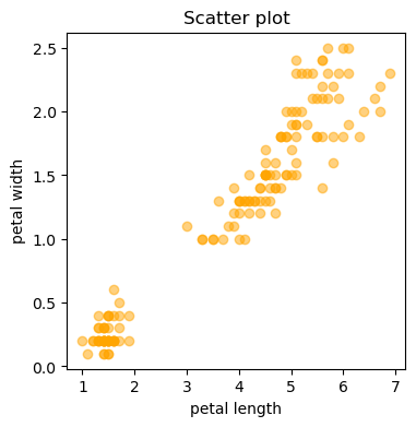
散布図を描いて相関を確認します
plt.figure(figsize = (4,4))
plt.scatter(X,y, color = 'orange', alpha = .5)
plt.title('Scatter plot')
plt.xlabel('petal length')
plt.ylabel('petal width')
plt.show()
# 学習データと検証データに分割
X_train, X_test, y_train, y_test = train_test_split(X, y, test_size=0.3, random_state=1,)
lr = LinearRegression()
lr.fit(X_train, y_train)
print(lr.score(X_test, y_test)) # R2
y_predicted = lr.predict(X_test)
print(mean_squared_error(y_test, y_predicted))
0.9217091797032136
0.039618634662187104
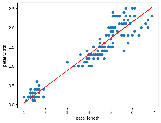
次に、学習された回帰モデルをプロットすることで、petal_lengthとpetal_widthの実際のデータをうまく表現できているかを確認します。
plt.scatter(X,y)
plt.plot(X, lr.predict(X), color = 'red') # 回帰直線をプロット
plt.xlabel('petal length')
plt.ylabel('petal width')
plt.show()
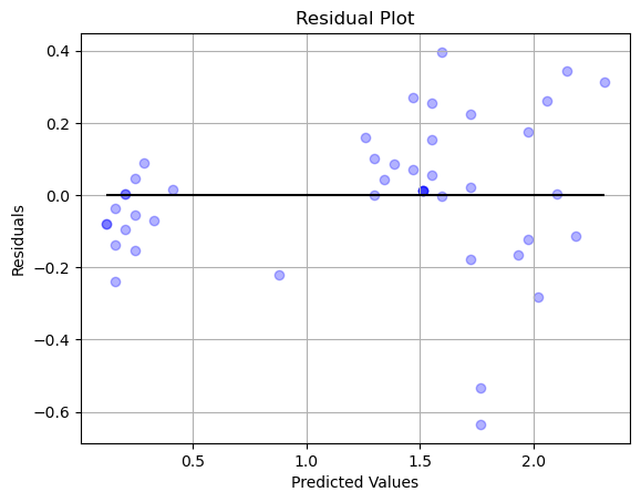
モデルがデータをうまく表現できているかを確認する方法としては、残差のプロットも有効です。
残差が0の周辺でランダムにばらついていれば、うまく表現できていて、そうでない別のパターン等がある場合は、モデルでは説明しきれていない情報があることが示唆されます。
plt.scatter(y_predicted, y_predicted - y_test, color = 'blue', alpha = 0.3)      # 残差をプロット
plt.hlines(y = 0, xmin = min(y_predicted), xmax = max(y_predicted), color = 'black') # x軸に沿った直線をプロット
plt.title('Residual Plot')
plt.xlabel('Predicted Values')
plt.ylabel('Residuals')
plt.grid()
plt.show()